The Flexible Image Transport System (FITS) is the standard format for representing images and data in Astronomy.

The KStars FITS Viewer tool is integrated with Ekos for seamless display of captured FITS images. It can be used as a standalone tool or embedded within Ekos modules. To open a FITS file, select Open FITS... from the File menu, or press Ctrl+O.

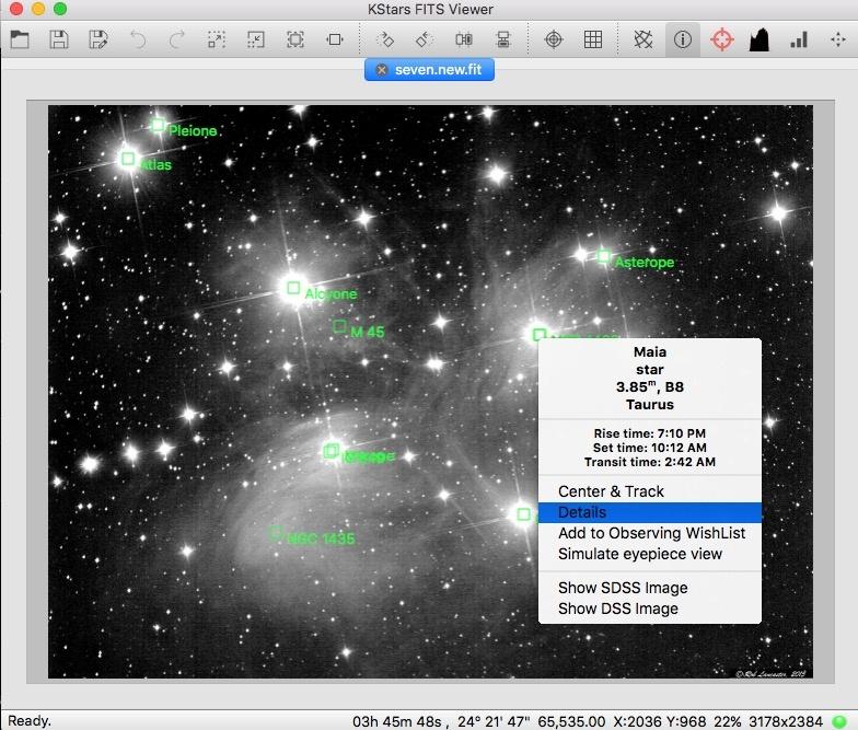
In addition to image display, the viewer can process World-Coordinate-System (WCS) header if present within the FITS file and provides useful information regarding the objects found within the image, equatorial grid overlay, popup menu, and the ability to slew the mount (if connected) to any point within the image.

Several filters can be applied to enhance the image include auto stretch and high contrast. Depending on the image size, these operation can take a few seconds to complete. The bottom status bar displays the current pixel value and current X & Y coordinates of the mouse pointer within the image. Furthermore, it includes the current zoom level and the image resolution.

When loading a bayered image, the viewer can automatically debayer the image if Auto Debayer is checked in the FITS Settings. The debayering operation fetches the bayer pattern (e.g. RGGB) from the FITS header. If none exists, you can alter the debaying algorithm and pattern from the File menu or by using the Ctrl+D shortcut.

Since operations such as auto debayering and auto WCS are computionality expensive and stress the processor on low-powered embedded devices, you can toggle their behavior in KStars Settings --> FITS.

 

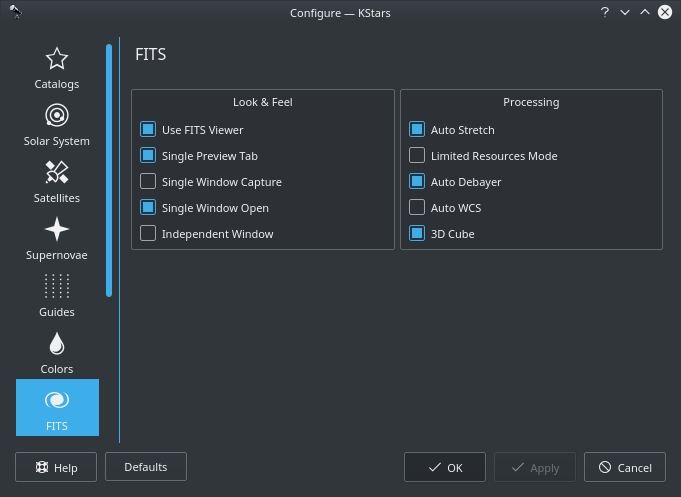
Hovering over any option shall display a detailed tooltip that explain its function.

Features

• Support for 8, 16, 32, IEEE -32, and IEEE -64 bits formats.

• Support Color FITS images (3D Cubes) and Bayered FITS images.

• Histogram with linear, logarithmic, and square-root scales.

• Brightness/Contrast controls.

• Pan and Zoom.

• Auto levels.

• Statistics.

• Rectangular and Equatorial Grids (if WCS info is present).

• Detection and highlight of stars.

• FITS header query.

• Undo/Redo.

Histogram

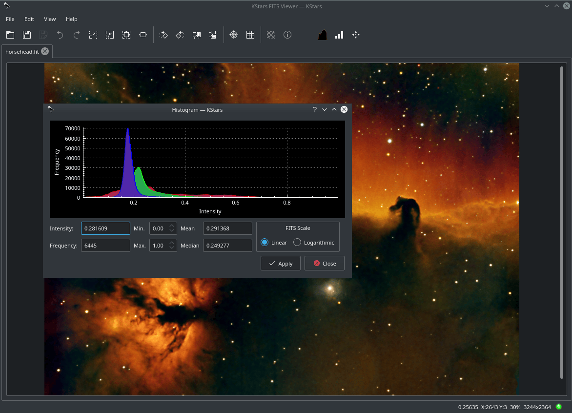
Displays multi-channel FITS histogram. The user can rescale the image by optionally defining an upper and lower limit for the cutoff region. The rescaling operation (linear, logarithmic, or square-root) may then be applied to the region enclosed by the upper and lower limits.

FITS Header

Displays a read-only table listing FITS header keywords and values.

Statistics

Provides simple statistics for minimum and maximum pixel values and their respective locations. FITS depth, dimension, mean, and standard deviation.

Embedded FITS Viewer

In Ekos Focus, Guide, and Align 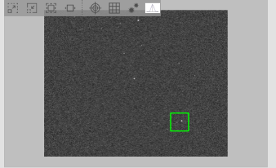modules, captured images are displayed in the embedded FITS Viewer. The embedded viewer includes a floating bar that can be used to perform several functions:

• Zoom Out
• Zoom In
• Default Zoom
• Zoom To Fit
• Toggle Cross Hairs
• Toggle Pixel Gridlines
• Toggle Detected Stars: Highlight detected stars with red circles.
• Star Profile: View detailed 3D star profile.

The floating bar is automatically hidden once the mouse leaves the embedded viewer area. You can use the mouse to pan and zoom just like the standalone FITSViewer tool. The green tracking box can be used to select a specific star or region within the image, for example, to select a guide star.

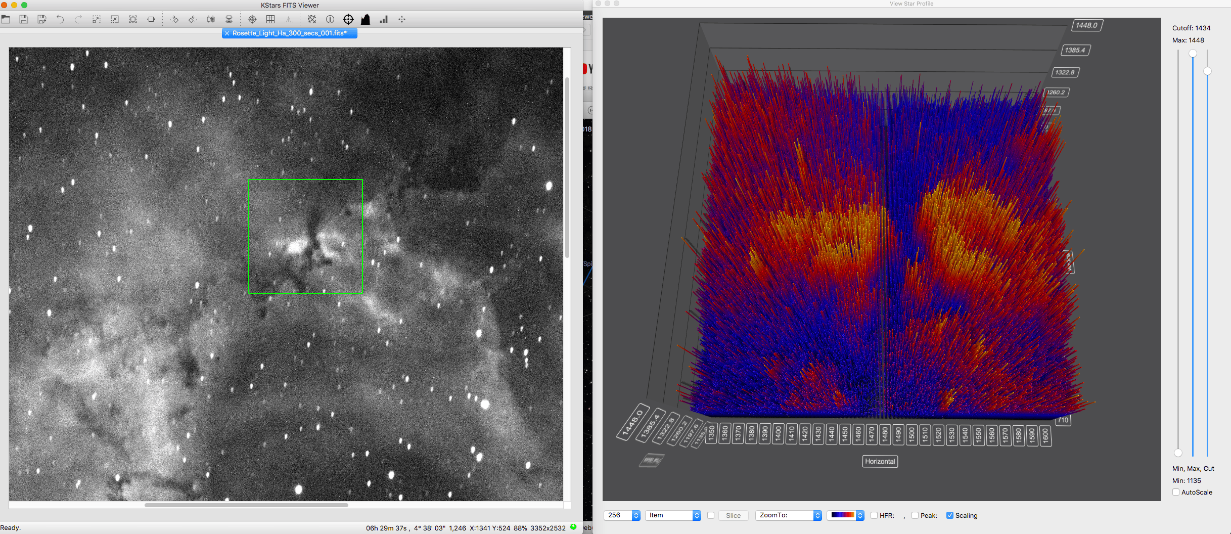
3D Star Profile & Data Visualization Tool

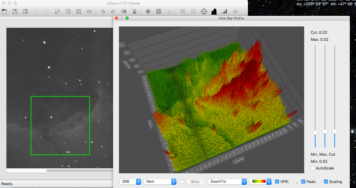
The 3D data visualization tool can plot 3D graphs of the selected region of the image. This is particularly useful for astrophotographers who want to visualize the profile of a star they are considering focusing or guiding on. For scientists, it enables them to examine a cross section of the data to understand the relative brightness of different objects in the image. Additionally, it empowers imagers who want to visually see what is going on in their data collection in a new way.

To use the new feature, the user needs to select the View Star Profile Icon in one of the Ekos Module Views, or in the Fitsviewer. Then, the region selected in the green tracking box will show up in the 3D graph as shown above. The user will then have one of the following toolbars at the bottom.

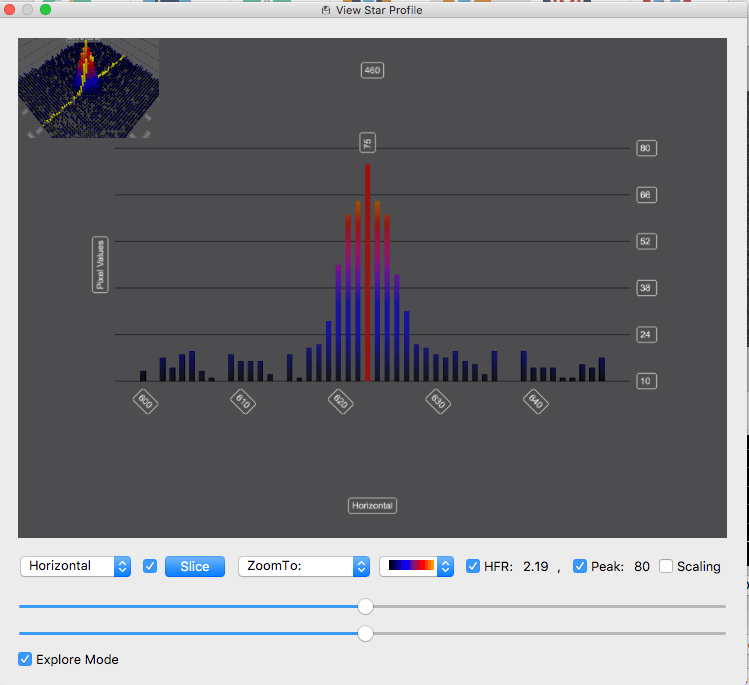
At the far left, the sample size combo box will let the user select the size of the image crop shown in the graph. This option is only available in the Summary Screen, the Align Module, and the FITSViewer. The second combo box lets the user control whether they are selecting an individual item, or a row, or a column of pixels. The slice button will be enabled if the user selects “Row” or “Column.” It will put the graph in slice mode so that the user can see a cross section view of the image. Third, is a check box that will open up two sliders that will let the user drag the slider to change the selection. This is extremely useful in the slide mode to change the selected point and to move the cross section around the graph. It is also useful in the normal view when in “Explore Mode” so that the user can zoom around the image examining the pixels.

Then the user has the “Zoom To” combo box, which the user can use to zoom the graph to different preset locations. Next is the combo box that lets the user select the color scheme of the graph. Then are the HFR and the Peak checkboxes, which will both turn on the HFR and Peak labels on each found star in the image, but will also display one of them at the bottom of the screen. And finally comes the Scaling checkbox, which enables the Scaling Side Panel. In that panel are three sliders, one to control the minimum value displayed on the graph or “black point”, one to control the maximum value displayed in the graph or the “white point,” and a third that is disabled by default that lets the user control the cutoff value for data displayed on the graph.

This third slider is very useful to get really big peaks out of the way so you can study the finer details in the image. There is a checkbox at the top to enable/disable the cutoff slider. And finally at the bottom of the sliders is the “Auto scale” button. This will auto scale the sliders as you sample different areas in the image. It will not only optimize the display of the data, but will also affect the minimum and maximum points of the slider. If you disable auto scale, then as you sample different parts of the image, they will be displayed at the same scale. A particularly useful way to use this is to select an area of your image using auto scale, tweak the min, max, and cutoff sliders to your liking, and then turn off the auto scale feature to explore other areas of the graph.